Chapter 5 Joining Data
Summary
| Mutating joins | Filtering joins | |
|---|---|---|
| descriptions | combine the variables from two tables. | keeps or removes observations from the first table, but it doesn’t add new variables. |
| verbs |
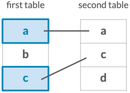
Keeps only observations which match exactly between two tables.
Keep all observations from the first table in your joins.
Keep all observations from the second table in your joins.
Keep all observations from both tables.
|
Filter the first table for observations which also exist in the second table.
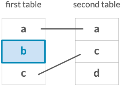
Filter the first table for observations that do not exist in the second table.
|
Load datasets from Rebrickable. And library package.
library(tidyverse)

sets <- read_csv("data/lego/sets.csv")
themes <- read_csv("data/lego/themes.csv")
parts <- read_csv("data/lego/parts.csv")
part_categories <- read_csv("data/lego/part_categories.csv")
inventories <- read_csv("data/lego/inventories.csv")
inventory_parts <- read_csv("data/lego/inventory_parts.csv")
colors <- read_csv("data/lego/colors.csv")
5.1 Inner join
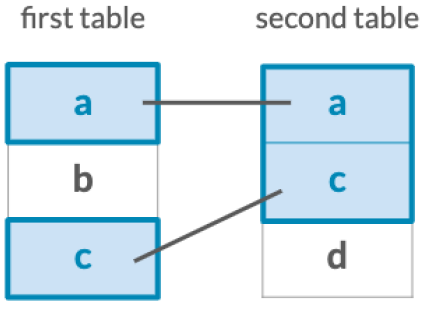
An inner join keeps an observation only if it has an exact match between the first and the second tables.
by argument tells inner join how to match the tables. If there are same variables name in each table, suffix argument can change variable name by adding characters you assign.
Syntax:
table1 %>%
    inner_join(table2, by = c(table2_key = table1_key), suffix = c("_chr1", "_chr2"))

# For example
sets %>%
    inner_join(themes, by = c("theme_id" = "id"), suffix = c("_set", "_theme"))
5.1.1 Join by keys
# Add the correct verb, table, and joining column
parts %>%
  inner_join(part_categories, by = c("part_cat_id" = "id"))
## # A tibble: 52,600 × 5
## part_num name.x part_cat_id part_material name.y
## <chr> <chr> <dbl> <chr> <chr>
## 1 003381 Sticker Sheet for Set 663-1 58 Plastic Stick…
## 2 003383 Sticker Sheet for Sets 618-1, 628-2 58 Plastic Stick…
## 3 003402 Sticker Sheet for Sets 310-3, 311-… 58 Plastic Stick…
## 4 003429 Sticker Sheet for Set 1550-1 58 Plastic Stick…
## 5 003432 Sticker Sheet for Sets 357-1, 355-… 58 Plastic Stick…
## 6 003434 Sticker Sheet for Set 575-2, 653-1… 58 Plastic Stick…
## 7 003435 Sticker Sheet for Set 687-1 58 Plastic Stick…
## 8 003436 Sticker Sheet for Set 180-1 58 Plastic Stick…
## 9 003437 Sticker Sheet for Set 181-1 58 Plastic Stick…
## 10 003438 Sticker Sheet for Set 131-1 58 Plastic Stick…
## # ℹ 52,590 more rows# Use the suffix argument to replace .x and .y suffixes
parts %>%
inner_join(part_categories, by = c("part_cat_id" = "id"),
suffix = c("_part", "_category"))## # A tibble: 52,600 × 5
## part_num name_part part_cat_id part_material name_category
## <chr> <chr> <dbl> <chr> <chr>
## 1 003381 Sticker Sheet for Set 663-1 58 Plastic Stickers
## 2 003383 Sticker Sheet for Sets 618-… 58 Plastic Stickers
## 3 003402 Sticker Sheet for Sets 310-… 58 Plastic Stickers
## 4 003429 Sticker Sheet for Set 1550-1 58 Plastic Stickers
## 5 003432 Sticker Sheet for Sets 357-… 58 Plastic Stickers
## 6 003434 Sticker Sheet for Set 575-2… 58 Plastic Stickers
## 7 003435 Sticker Sheet for Set 687-1 58 Plastic Stickers
## 8 003436 Sticker Sheet for Set 180-1 58 Plastic Stickers
## 9 003437 Sticker Sheet for Set 181-1 58 Plastic Stickers
## 10 003438 Sticker Sheet for Set 131-1 58 Plastic Stickers
## # ℹ 52,590 more rows5.1.2 Join with a one-to-many relationship
This is an example of a one-to-many relationship. And by the same variable. Notice that the table increased in the number of rows after the join.
# Combine the parts and inventory_parts tables
parts %>%
    inner_join(inventory_parts, by = "part_num")
## # A tibble: 1,179,869 × 9
## part_num name part_cat_id part_material inventory_id color_id quantity
## <chr> <chr> <dbl> <chr> <dbl> <dbl> <dbl>
## 1 003381 Sticker Sh… 58 Plastic 15865 9999 1
## 2 003383 Sticker Sh… 58 Plastic 8376 9999 1
## 3 003383 Sticker Sh… 58 Plastic 11738 9999 1
## 4 003402 Sticker Sh… 58 Plastic 470 9999 1
## 5 003402 Sticker Sh… 58 Plastic 885 9999 1
## 6 003402 Sticker Sh… 58 Plastic 12659 9999 1
## 7 003429 Sticker Sh… 58 Plastic 3993 9999 1
## 8 003432 Sticker Sh… 58 Plastic 8191 9999 1
## 9 003434 Sticker Sh… 58 Plastic 8756 9999 1
## 10 003434 Sticker Sh… 58 Plastic 12826 9999 1
## # ℹ 1,179,859 more rows
## # ℹ 2 more variables: is_spare <lgl>, img_url <chr>5.1.3 Join in either direction
An inner_join works the same way with either table in either position. The table that is specified first is arbitrary, since you will end up with the same information in the resulting table either way.(table先後順序不同所得結果一樣)
# Combine the parts and inventory_parts tables
inventory_parts %>%
  inner_join(parts, by = "part_num")
## # A tibble: 1,179,869 × 9
## inventory_id part_num color_id quantity is_spare img_url name part_cat_id
## <dbl> <chr> <dbl> <dbl> <lgl> <chr> <chr> <dbl>
## 1 1 48379c01 72 1 FALSE https:… Larg… 41
## 2 1 48395 7 1 FALSE https:… Spor… 27
## 3 1 stickerupn… 9999 1 FALSE <NA> Stic… 58
## 4 1 upn0342 0 1 FALSE <NA> Spor… 27
## 5 1 upn0350 25 1 FALSE <NA> Spor… 13
## 6 3 2343 47 1 FALSE https:… Equi… 27
## 7 3 3003 29 1 FALSE https:… Bric… 11
## 8 3 30176 2 1 FALSE https:… Plan… 28
## 9 3 3020 15 1 FALSE https:… Plat… 14
## 10 3 3022 15 2 FALSE https:… Plat… 14
## # ℹ 1,179,859 more rows
## # ℹ 1 more variable: part_material <chr>This is the same join as the last exercise, but the order of the tables is reversed. For an inner_join, either direction will yield a table that contains the same information! Note that the columns will appear in a different order depending on which table comes first.
5.1.4 Join three or more tables
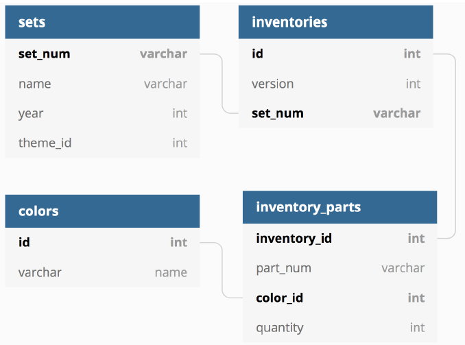
sets %>%
  # Add inventories using an inner join
  inner_join(inventories, by = "set_num") %>%
  # Add inventory_parts using an inner join
  inner_join(inventory_parts, by = c("id" = "inventory_id"))
## # A tibble: 1,113,729 × 13
## set_num name year theme_id num_parts img_url.x id version part_num
## <chr> <chr> <dbl> <dbl> <dbl> <chr> <dbl> <dbl> <chr>
## 1 001-1 Gears 1965 1 43 https://cdn.re… 24696 1 132a
## 2 001-1 Gears 1965 1 43 https://cdn.re… 24696 1 3020
## 3 001-1 Gears 1965 1 43 https://cdn.re… 24696 1 3062c
## 4 001-1 Gears 1965 1 43 https://cdn.re… 24696 1 3404bc01
## 5 001-1 Gears 1965 1 43 https://cdn.re… 24696 1 36
## 6 001-1 Gears 1965 1 43 https://cdn.re… 24696 1 7039
## 7 001-1 Gears 1965 1 43 https://cdn.re… 24696 1 7049bc01
## 8 001-1 Gears 1965 1 43 https://cdn.re… 24696 1 715
## 9 001-1 Gears 1965 1 43 https://cdn.re… 24696 1 741
## 10 001-1 Gears 1965 1 43 https://cdn.re… 24696 1 742
## # ℹ 1,113,719 more rows
## # ℹ 4 more variables: color_id <dbl>, quantity <dbl>, is_spare <lgl>,
## # img_url.y <chr># Count the number of colors and sort
sets %>%
inner_join(inventories, by = "set_num") %>%
inner_join(inventory_parts, by = c("id" = "inventory_id")) %>%
inner_join(colors, by = c("color_id" = "id"),
suffix = c("_set", "_color")) %>%
count(name_color) %>%
arrange(desc(n))## # A tibble: 250 × 2
## name_color n
## <chr> <int>
## 1 Black 198156
## 2 White 126555
## 3 Light Bluish Gray 121453
## 4 Dark Bluish Gray 89669
## 5 Red 84521
## 6 Yellow 57755
## 7 Blue 45305
## 8 Reddish Brown 37606
## 9 Tan 34831
## 10 Light Gray 28104
## # ℹ 240 more rows5.2 Left & Right Joins
5.2.1 Left join
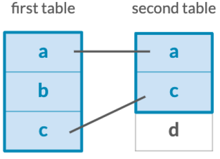
Left joining two sets by part and color
Each of these observations isn’t just a part, but a combination of a part and a color. Notice, you can specify this with by = c("var1", "var2"). That specifies we want to join on both columns.
# Prepare tables
inventory_parts_joined <- inventories %>%
    inner_join(inventory_parts, by = c("id" = "inventory_id")) %>%
    select(-id, -version) %>%
    arrange(desc(quantity))

millennium_falcon <- inventory_parts_joined %>%
  filter(set_num == "7965-1")

star_destroyer <- inventory_parts_joined %>%
  filter(set_num == "75190-1")

# Combine the star_destroyer and millennium_falcon tables
millennium_falcon %>%
  left_join(star_destroyer, by = c("part_num", "color_id"),
            suffix = c("_falcon", "_star_destroyer"))
## Warning in left_join(., star_destroyer, by = c("part_num", "color_id"), : Detected an unexpected many-to-many
## relationship between `x` and `y`.
## ℹ Row 4 of `x` matches multiple rows in `y`.
## ℹ Row 3 of `y` matches multiple rows in `x`.
## ℹ If a many-to-many relationship is expected,
## set `relationship = "many-to-many"` to
## silence this warning.## # A tibble: 247 × 10
## set_num_falcon part_num color_id quantity_falcon is_spare_falcon
## <chr> <chr> <dbl> <dbl> <lgl>
## 1 7965-1 63868 71 62 FALSE
## 2 7965-1 3023 0 60 FALSE
## 3 7965-1 3021 72 46 FALSE
## 4 7965-1 2780 0 37 FALSE
## 5 7965-1 2780 0 37 FALSE
## 6 7965-1 60478 72 36 FALSE
## 7 7965-1 6636 71 34 FALSE
## 8 7965-1 3009 71 28 FALSE
## 9 7965-1 3665 71 22 FALSE
## 10 7965-1 2412b 72 20 FALSE
## # ℹ 237 more rows
## # ℹ 5 more variables: img_url_falcon <chr>, set_num_star_destroyer <chr>,
## # quantity_star_destroyer <dbl>, is_spare_star_destroyer <lgl>,
## # img_url_star_destroyer <chr>Left joining two sets by color
# Aggregate Millennium Falcon for the total quantity in each part
millennium_falcon_colors <- millennium_falcon %>%
  group_by(color_id) %>%
  summarize(total_quantity = sum(quantity))

# Aggregate Star Destroyer for the total quantity in each part
star_destroyer_colors <- star_destroyer %>%
  group_by(color_id) %>%
  summarize(total_quantity = sum(quantity))

# Left join the Millennium Falcon colors to the Star Destroyer colors
millennium_falcon_colors %>%
  left_join(star_destroyer_colors, by = "color_id",
            suffix = c("_falcon", "_star_destroyer"))
## # A tibble: 19 × 3
## color_id total_quantity_falcon total_quantity_star_destroyer
## <dbl> <dbl> <dbl>
## 1 0 196 327
## 2 1 15 24
## 3 4 17 56
## 4 14 3 5
## 5 15 12 13
## 6 19 91 13
## 7 28 3 16
## 8 33 5 NA
## 9 36 1 14
## 10 41 6 16
## 11 47 5 NA
## 12 70 6 1
## 13 71 586 533
## 14 72 282 373
## 15 80 3 NA
## 16 179 2 NA
## 17 320 12 2
## 18 1103 1 NA
## 19 9999 1 1Finding an observation that doesn’t have a match
For example, the inventories table has a version column, for when a LEGO kit gets some kind of change or upgrade. It would be fair to assume that all sets (which joins well with inventories) would have at least a version 1.
And use the replace_na, which takes a list of column names and the values with which NAs should be replaced, to clean up our table.
replace_na(list(colname = replace_value))inventory_version_1 <- inventories %>%
filter(version == 1)
colnames(inventory_version_1)## [1] "id" "version" "set_num"colnames(sets)## [1] "set_num" "name" "year" "theme_id" "num_parts" "img_url"# Join versions to sets
sets %>%
left_join(inventory_version_1, by = "set_num") %>%
# Filter for where version is na
filter(is.na(version)) %>%
# Use replace_na to replace missing values in the version column
replace_na(list(version = 0))## # A tibble: 3 × 8
## set_num name year theme_id num_parts img_url id version
## <chr> <chr> <dbl> <dbl> <dbl> <chr> <dbl> <dbl>
## 1 10875-1 Cargo Train 2018 634 105 https:… NA 0
## 2 76081-1 The Milano vs. The Abi… 2017 704 462 https:… NA 0
## 3 S1-1 Baseplate with steerin… 1970 453 1 https:… NA 05.2.2 Right join
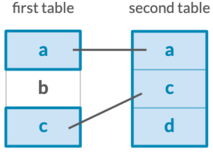
In this exercise, we’ll count the part_cat_id from parts, before using a right_join to join with part_categories. The reason we do this is because we don’t only want to know the count of part_cat_id in parts, but we also want to know if there are any part_cat_ids not present in parts.
parts %>%
  # Count the part_cat_id
  count(part_cat_id) %>%
  # Right join part_categories
  right_join(part_categories, by = c("part_cat_id" = "id")) %>%
  # Filter for NA
  filter(is.na(n))
## # A tibble: 0 × 3
## # ℹ 3 variables: part_cat_id <dbl>, n <int>, name <chr>Joining tables to themselves
In the themes table, you’ll notice there is both an id column and a parent_id column. Keeping that in mind, you can join the themes table to itself to determine the parent-child relationships that exist for different themes.
- Joining themes to their children
In this exercise, you’ll try a similar approach of joining themes to their own children, which is similar but reversed.
themes %>%
  # Inner join the themes table
  inner_join(themes, by = c("id" = "parent_id"), suffix = c("_parent", "_child")) %>%
  # Filter for the "Harry Potter" parent name
  filter(name_parent == "Harry Potter")
## # A tibble: 1 × 5
## id name_parent parent_id id_child name_child
## <dbl> <chr> <dbl> <dbl> <chr>
## 1 246 Harry Potter NA 667 Fantastic Beasts- Joining themes to their grandchildren
Some themes actually have grandchildren: their children’s children. Here, we can inner join themes to a filtered version of itself again to establish a connection between our last join’s children and their children.
# Join themes to itself again to find the grandchild relationships
themes %>%
  inner_join(themes, by = c("id" = "parent_id"), suffix = c("_parent", "_child")) %>%
  inner_join(themes, by = c("id_child" = "parent_id"), suffix = c("_parent", "_grandchild"))
## # A tibble: 23 × 7
## id_parent name_parent parent_id id_child name_child id_grandchild name
## <dbl> <chr> <dbl> <dbl> <chr> <dbl> <chr>
## 1 206 Seasonal NA 207 Advent 208 City
## 2 206 Seasonal NA 207 Advent 209 Star Wars
## 3 206 Seasonal NA 207 Advent 210 Belville
## 4 206 Seasonal NA 207 Advent 211 Castle
## 5 206 Seasonal NA 207 Advent 212 Classic Ba…
## 6 206 Seasonal NA 207 Advent 213 Clikits
## 7 206 Seasonal NA 207 Advent 214 Creator
## 8 206 Seasonal NA 207 Advent 215 Pirates
## 9 206 Seasonal NA 207 Advent 216 Friends
## 10 206 Seasonal NA 207 Advent 710 Harry Pott…
## # ℹ 13 more rows- Left joining a table to itself
themes %>%
  # Left join the themes table to its own children
  left_join(themes, by = c("id" = "parent_id"), suffix = c("_parent", "_child")) %>%
  # Filter for themes that have no child themes
  filter(is.na(name_child))
## # A tibble: 412 × 5
## id name_parent parent_id id_child name_child
## <dbl> <chr> <dbl> <dbl> <chr>
## 1 3 Competition 1 NA <NA>
## 2 4 Expert Builder 1 NA <NA>
## 3 16 RoboRiders 1 NA <NA>
## 4 17 Speed Slammers 1 NA <NA>
## 5 18 Star Wars 1 NA <NA>
## 6 19 Supplemental 1 NA <NA>
## 7 20 Throwbot Slizer 1 NA <NA>
## 8 21 Universal Building Set 1 NA <NA>
## 9 23 Basic Model 22 NA <NA>
## 10 35 Bricks & More 34 NA <NA>
## # ℹ 402 more rows5.3 Full, Semi & Anti Joins
5.3.1 Full join
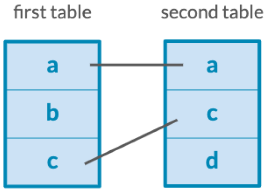
# keep all both
batmobile %>%
  full_join(batwing, by = c("part_num", "color_id"),
  suffix = c("_batmobile", "_batwing"))
Differences between Batman and Star Wars
Now, you’ll compare two themes, each of which is made up of many sets. Since each theme is made up of many sets, combining these tables is the first step towards being able to compare different themes.
inventory_parts_joined <- inventories %>%
  inner_join(inventory_parts, by = c("id" = "inventory_id")) %>%
  arrange(desc(quantity)) %>%
  select(-id, -version)
# Start with inventory_parts_joined table
inventory_sets_themes <- inventory_parts_joined %>%
# Combine with the sets table
inner_join(sets, by = "set_num") %>%
# Combine with the themes table
inner_join(themes, by = c("theme_id" = "id"), suffix = c("_set", "_theme"))
inventory_sets_themes## # A tibble: 1,113,729 × 13
## set_num part_num color_id quantity is_spare img_url.x name_set year theme_id
## <chr> <chr> <dbl> <dbl> <lgl> <chr> <chr> <dbl> <dbl>
## 1 31203-1 6141 15 3064 FALSE https://… World M… 2021 709
## 2 31203-1 98138 3 1879 FALSE https://… World M… 2021 709
## 3 31203-1 98138 322 1607 FALSE https://… World M… 2021 709
## 4 k34432… 3024 15 1440 FALSE https://… Lego Mo… 2003 277
## 5 k34433… 3024 15 1170 FALSE https://… Lego Mo… 2003 277
## 6 31203-1 98138 27 1060 FALSE https://… World M… 2021 709
## 7 40179-1 3024 14 900 FALSE https://… Persona… 2016 277
## 8 40179-1 3024 71 900 FALSE https://… Persona… 2016 277
## 9 40179-1 3024 72 900 FALSE https://… Persona… 2016 277
## 10 40179-1 3024 15 900 FALSE https://… Persona… 2016 277
## # ℹ 1,113,719 more rows
## # ℹ 4 more variables: num_parts <dbl>, img_url.y <chr>, name_theme <chr>,
## # parent_id <dbl>Aggregating each theme
Before doing this comparison, you’ll want to aggregate the data to learn more about the pieces that are a part of each theme, as well as the colors of those pieces.
# filtered for each theme
batman <- inventory_sets_themes %>%
  filter(name_theme == "Batman")

star_wars <- inventory_sets_themes %>%
  filter(name_theme == "Star Wars")

# Count the part number and color id, weight by quantity
batman_parts <- batman %>%
    count(part_num, color_id, wt = quantity); batman_parts
## # A tibble: 3,455 × 3
## part_num color_id n
## <chr> <dbl> <dbl>
## 1 10100596 9999 1
## 2 10104735 9999 1
## 3 10104995 9999 1
## 4 10172 179 1
## 5 10172 297 1
## 6 10187 179 3
## 7 10187 297 3
## 8 10190 0 8
## 9 10201 4 3
## 10 10201 14 5
## # ℹ 3,445 more rowsstar_wars_parts <- star_wars %>%
count(part_num, color_id, wt = quantity); star_wars_parts## # A tibble: 9,081 × 3
## part_num color_id n
## <chr> <dbl> <dbl>
## 1 01571 9999 1
## 2 01709 9999 1
## 3 01832 9999 1
## 4 10001722 9999 1
## 5 10001831 9999 1
## 6 10050 1063 4
## 7 10050 1103 1
## 8 10100101 9999 1
## 9 10100763 9999 1
## 10 10100764 9999 1
## # ℹ 9,071 more rowsFull joining Batman and Star Wars LEGO parts
Now that you’ve got separate tables for the pieces in the batman and star_wars themes, you’ll want to be able to combine them to see any similarities or differences between the two themes.
parts_joined <- batman_parts %>%
    # Combine the star_wars_parts table
    full_join(star_wars_parts, by = c("part_num", "color_id"),
              suffix = c("_batman", "_star_wars")) %>%
    # Replace NAs with 0s in the n_batman and n_star_wars columns
    replace_na(list(n_batman = 0,
                    n_star_wars = 0))
parts_joined
## # A tibble: 9,964 × 4
## part_num color_id n_batman n_star_wars
## <chr> <dbl> <dbl> <dbl>
## 1 10100596 9999 1 0
## 2 10104735 9999 1 0
## 3 10104995 9999 1 0
## 4 10172 179 1 0
## 5 10172 297 1 0
## 6 10187 179 3 0
## 7 10187 297 3 3
## 8 10190 0 8 3
## 9 10201 4 3 7
## 10 10201 14 5 2
## # ℹ 9,954 more rowsComparing Batman and Star Wars LEGO parts
However, we have more information about each of these parts that we can gain by combining this table with some of the information we have in other tables.
parts_joined %>%
  # Sort the number of star wars pieces in descending order
  arrange(desc(n_star_wars)) %>%
  # Join the colors table to the parts_joined table
  inner_join(colors, by = c("color_id" = "id")) %>%
  # Join the parts table to the previous join
  inner_join(parts, by = "part_num", suffix = c("_color", "_part"))
## # A tibble: 9,964 × 10
## part_num color_id n_batman n_star_wars name_color rgb is_trans name_part
## <chr> <dbl> <dbl> <dbl> <chr> <chr> <lgl> <chr>
## 1 2780 0 377 5200 Black 0513… FALSE Technic …
## 2 4274 1 166 2052 Blue 0055… FALSE Technic …
## 3 3023 71 101 1923 Light Bluish… A0A5… FALSE Plate 1 …
## 4 3023 72 170 1724 Dark Bluish … 6C6E… FALSE Plate 1 …
## 5 3023 0 240 1457 Black 0513… FALSE Plate 1 …
## 6 43093 1 95 1394 Blue 0055… FALSE Technic …
## 7 6141 36 86 1246 Trans-Red C91A… TRUE Plate Ro…
## 8 2412b 72 83 1245 Dark Bluish … 6C6E… FALSE Tile Spe…
## 9 6141 72 94 1178 Dark Bluish … 6C6E… FALSE Plate Ro…
## 10 6558 1 33 1133 Blue 0055… FALSE Technic …
## # ℹ 9,954 more rows
## # ℹ 2 more variables: part_cat_id <dbl>, part_material <chr>5.3.2 Semi & Anti joins
Something within one set but not another
Determine which parts are in both the batwing and batmobile sets, and which sets are in one, but not the other.
# Two sets
batmobile <- inventory_parts_joined %>%
  filter(set_num == "7784-1") %>%
  select(-set_num)

batwing <- inventory_parts_joined %>%
  filter(set_num == "70916-1") %>%
  select(-set_num)

# Filter the batwing set for parts that are also in the batmobile set
batwing %>%
  semi_join(batmobile, by = "part_num")
## # A tibble: 142 × 5
## part_num color_id quantity is_spare img_url
## <chr> <dbl> <dbl> <lgl> <chr>
## 1 3023 0 22 FALSE https://cdn.rebrickable.com/media/parts/…
## 2 3024 0 22 FALSE https://cdn.rebrickable.com/media/parts/…
## 3 3623 0 20 FALSE https://cdn.rebrickable.com/media/parts/…
## 4 2780 0 17 FALSE https://cdn.rebrickable.com/media/parts/…
## 5 3666 0 16 FALSE https://cdn.rebrickable.com/media/parts/…
## 6 3710 0 14 FALSE https://cdn.rebrickable.com/media/parts/…
## 7 6141 4 12 FALSE https://cdn.rebrickable.com/media/parts/…
## 8 2412b 71 10 FALSE https://cdn.rebrickable.com/media/parts/…
## 9 6141 72 10 FALSE https://cdn.rebrickable.com/media/parts/…
## 10 6558 1 9 FALSE https://cdn.rebrickable.com/media/parts/…
## # ℹ 132 more rows# Filter the batwing set for parts that aren't in the batmobile set
batwing %>%
anti_join(batmobile, by = "part_num")## # A tibble: 181 × 5
## part_num color_id quantity is_spare img_url
## <chr> <dbl> <dbl> <lgl> <chr>
## 1 11477 0 18 FALSE https://cdn.rebrickable.com/media/parts/…
## 2 99207 71 18 FALSE https://cdn.rebrickable.com/media/parts/…
## 3 22385 0 14 FALSE https://cdn.rebrickable.com/media/parts/…
## 4 99563 0 13 FALSE https://cdn.rebrickable.com/media/parts/…
## 5 10247 72 12 FALSE https://cdn.rebrickable.com/media/parts/…
## 6 2877 72 12 FALSE https://cdn.rebrickable.com/media/parts/…
## 7 61409 72 12 FALSE https://cdn.rebrickable.com/media/parts/…
## 8 11153 0 10 FALSE https://cdn.rebrickable.com/media/parts/…
## 9 98138 46 10 FALSE https://cdn.rebrickable.com/media/parts/…
## 10 2419 72 9 FALSE https://cdn.rebrickable.com/media/parts/…
## # ℹ 171 more rowsWhat colors are included in at least one set?
you could also use a filtering join like semi_join to find out which colors ever appear in any inventory part.
# Use inventory_parts to find colors included in at least one set
colors %>%
  semi_join(inventory_parts, by = c("id" = "color_id"))
## # A tibble: 250 × 4
## id name rgb is_trans
## <dbl> <chr> <chr> <lgl>
## 1 -1 [Unknown] 0033B2 FALSE
## 2 0 Black 05131D FALSE
## 3 1 Blue 0055BF FALSE
## 4 2 Green 237841 FALSE
## 5 3 Dark Turquoise 008F9B FALSE
## 6 4 Red C91A09 FALSE
## 7 5 Dark Pink C870A0 FALSE
## 8 6 Brown 583927 FALSE
## 9 7 Light Gray 9BA19D FALSE
## 10 8 Dark Gray 6D6E5C FALSE
## # ℹ 240 more rowsWhich set is missing version 1?
Let’s start by looking at the first version of each set to see if there are any sets that don’t include a first version.
# Use filter() to extract version 1
version_1_inventories <- inventories %>%
  filter(version == 1); version_1_inventories
## # A tibble: 35,612 × 3
## id version set_num
## <dbl> <dbl> <chr>
## 1 1 1 7922-1
## 2 3 1 3931-1
## 3 4 1 6942-1
## 4 15 1 5158-1
## 5 16 1 903-1
## 6 17 1 850950-1
## 7 19 1 4444-1
## 8 21 1 3474-1
## 9 22 1 30277-1
## 10 25 1 71012-11
## # ℹ 35,602 more rows# Use anti_join() to find which set is missing a version 1
sets %>%
anti_join(version_1_inventories, by = "set_num")## # A tibble: 3 × 6
## set_num name year theme_id num_parts img_url
## <chr> <chr> <dbl> <dbl> <dbl> <chr>
## 1 10875-1 Cargo Train 2018 634 105 https:…
## 2 76081-1 The Milano vs. The Abilisk 2017 704 462 https:…
## 3 S1-1 Baseplate with steering control tong… 1970 453 1 https:…This is likely a data quality issue, and anti_join is a great tool for finding problems like that.
5.3.3 Visualizing set differences
Aggregating sets to look at their differences
To compare two individual sets, and the kinds of LEGO pieces that comprise them, we’ll need to aggregate the data into separate themes.
In addition to being able to view the sets for Batman and Star Wars separately, adding the column also allowed us to be able to look at the fraction differences between the sets, rather than only being able to compare the numbers of pieces.
inventory_parts_themes <- inventories %>%
  inner_join(inventory_parts, by = c("id" = "inventory_id")) %>%
  arrange(desc(quantity)) %>%
  select(-id, -version) %>%
  inner_join(sets, by = "set_num") %>%
  inner_join(themes, by = c("theme_id" = "id"), suffix = c("_set", "_theme"))

batman_colors <- inventory_parts_themes %>%
  # Filter the inventory_parts_themes table for the Batman theme
  filter(name_theme == "Batman") %>%
  group_by(color_id) %>%
  summarize(total = sum(quantity)) %>%
  # Add a fraction column of the total divided by the sum of the total
  mutate(fraction = total / sum(total))

# Filter and aggregate the Star Wars set data; add a fraction column
star_wars_colors <- inventory_parts_themes %>%
  filter(name_theme == "Star Wars") %>%
  group_by(color_id) %>%
  summarize(total = sum(quantity)) %>%
  mutate(fraction = total / sum(total))
Combining sets
Prior to visualizing the data, you’ll want to combine these tables to be able to directly compare the themes’ colors.
batman_colors %>%
  # Join the Batman and Star Wars colors
  full_join(star_wars_colors, by = "color_id", suffix = c("_batman", "_star_wars")) %>%
  # Replace NAs in the total_batman and total_star_wars columns
  replace_na(list(total_batman = 0, total_star_wars = 0)) %>%
  inner_join(colors, by = c("color_id" = "id")) %>%
  # Create the difference and total columns
  mutate(difference = fraction_batman - fraction_star_wars,
         total = total_batman + total_star_wars) %>%
  # Filter for totals greater than 200
  filter(total >= 200)
## # A tibble: 42 × 10
## color_id total_batman fraction_batman total_star_wars fraction_star_wars
## <dbl> <dbl> <dbl> <dbl> <dbl>
## 1 0 9630 0.343 49016 0.184
## 2 1 495 0.0176 8643 0.0325
## 3 2 273 0.00972 1300 0.00489
## 4 4 889 0.0317 7203 0.0271
## 5 14 962 0.0343 4302 0.0162
## 6 15 755 0.0269 23618 0.0889
## 7 19 863 0.0307 11915 0.0448
## 8 25 166 0.00591 2151 0.00809
## 9 27 125 0.00445 615 0.00231
## 10 28 818 0.0291 5194 0.0195
## # ℹ 32 more rows
## # ℹ 5 more variables: name <chr>, rgb <chr>, is_trans <lgl>, difference <dbl>,
## # total <dbl>Visualizing the difference: Batman and Star Wars
Now you’ll create a bar plot with one bar for each color (name), showing the difference in fractions.
library(forcats)

colors_joined <- batman_colors %>%
  full_join(star_wars_colors, by = "color_id", suffix = c("_batman", "_star_wars")) %>%
  replace_na(list(total_batman = 0, total_star_wars = 0)) %>%
  inner_join(colors, by = c("color_id" = "id")) %>%
  mutate(difference = fraction_batman - fraction_star_wars,
         total = total_batman + total_star_wars) %>%
  filter(total >= 200) %>%
  replace_na(list(difference = 0)) %>%
  mutate(name = fct_reorder(name, difference))


# we need to add # to create our palette
colors_joined$rgb <- paste("#", colors_joined$rgb, sep="")
color_palette <- setNames(colors_joined$rgb, colors_joined$name)

# Create a bar plot using colors_joined and the name and difference columns
ggplot(colors_joined, aes(x = name, y = difference, fill = name)) +
  geom_col() +
  coord_flip() +
  scale_fill_manual(values = color_palette, guide = "none") +
  labs(y = "Difference: Batman - Star Wars")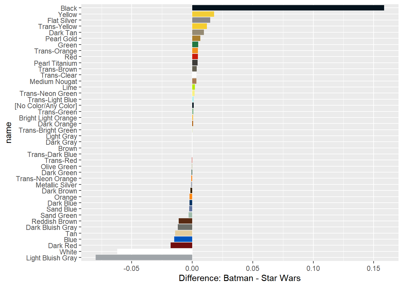
5.4 Case study: Joins on Stack Overflow Data
5.4.1 Load dataset
Three of the Stack Overflow survey datasets are questions, question_tags, and tags:
questions: an ID and the score, or how many times the question has been upvoted; the data only includes R-based questions.question_tags: a tag ID for each question and the question’s id.tags: a tag id and the tag’s name, which can be used to identify the subject of each question, such as ggplot2 or dplyr.
questions <- read_csv("data/stackoverflow/questions.csv")
question_tags <- read_csv("data/stackoverflow/question_tags.csv")
tags <- read_csv("data/stackoverflow/tags.csv")
answers <- read_csv("data/stackoverflow/answers.csv")

colnames(questions)
## [1] "id" "creation_date" "score"colnames(question_tags)## [1] "question_id" "tag_id"colnames(tags)## [1] "id" "tag_name"colnames(answers)## [1] "id" "creation_date" "question_id" "score"5.4.3 Joining questions and answers
5.4.3.1 Finding gaps between questions and answers
Now we’ll join together questions with answers so we can measure the time between questions and answers.
questions %>%
  # Inner join questions and answers with proper suffixes
  inner_join(answers, by = c("id" = "question_id"),
             suffix = c("_question", "_answer")) %>%
  # Subtract creation_date_question from creation_date_answer to create gap
  mutate(gap = as.integer(as.Date(creation_date_answer, format = "%m/%d/%Y") - as.Date(creation_date_question, format = "%m/%d/%Y")))
## Warning in inner_join(., answers, by = c(id = "question_id"), suffix = c("_question", : Detected an unexpected many-to-many
## relationship between `x` and `y`.
## ℹ Row 2 of `x` matches multiple rows in `y`.
## ℹ Row 118226 of `y` matches multiple rows in
## `x`.
## ℹ If a many-to-many relationship is expected,
## set `relationship = "many-to-many"` to
## silence this warning.## # A tibble: 592,547 × 7
## id creation_date_question score_question id_answer creation_date_answer
## <dbl> <chr> <dbl> <dbl> <chr>
## 1 22557677 3/21/2014 1 22560670 3/21/2014
## 2 22557707 3/21/2014 2 22558516 3/21/2014
## 3 22557707 3/21/2014 2 22558726 3/21/2014
## 4 22558084 3/21/2014 2 22558085 3/21/2014
## 5 22558084 3/21/2014 2 22606545 3/24/2014
## 6 22558084 3/21/2014 2 22610396 3/24/2014
## 7 22558084 3/21/2014 2 34374729 12/19/2015
## 8 22558395 3/21/2014 2 22559327 3/21/2014
## 9 22558395 3/21/2014 2 22560102 3/21/2014
## 10 22558395 3/21/2014 2 22560288 3/21/2014
## # ℹ 592,537 more rows
## # ℹ 2 more variables: score_answer <dbl>, gap <int>5.4.3.2 Joining question and answer counts
We can also determine how many questions actually yield answers. If we count the number of answers for each question, we can then join the answers counts with the questions table.
# Count and sort the question id column in the answers table
answer_counts <- answers %>%
  count(question_id, sort = TRUE)

# Combine the answer_counts and questions tables
question_answer_counts <- questions %>%
  left_join(answer_counts, by = c("id" = "question_id")) %>%
  # Replace the NAs in the n column
  replace_na(list(n = 0)); question_answer_counts
## # A tibble: 394,732 × 4
## id creation_date score n
## <dbl> <chr> <dbl> <int>
## 1 22557677 3/21/2014 1 1
## 2 22557707 3/21/2014 2 2
## 3 22558084 3/21/2014 2 4
## 4 22558395 3/21/2014 2 3
## 5 22558613 3/21/2014 0 1
## 6 22558677 3/21/2014 2 2
## 7 22558887 3/21/2014 8 1
## 8 22559180 3/21/2014 1 1
## 9 22559312 3/21/2014 0 1
## 10 22559322 3/21/2014 2 5
## # ℹ 394,722 more rows5.4.3.4 Average answers by question
You can use tagged_answers to determine, on average, how many answers each questions gets.
Some of the important variables from this table include: n, the number of answers for each question, and tag_name, the name of each tag associated with each question.
tagged_answers %>%
  # Aggregate by tag_name
  group_by(tag_name)  %>%
  # Summarize questions and average_answers
  summarize(questions = n(),
            average_answers = mean(n)) %>%
  # Sort the questions in descending order
  arrange(desc(questions))
## # A tibble: 7,841 × 3
## tag_name questions average_answers
## <chr> <int> <dbl>
## 1 ggplot2 42627 1.29
## 2 dataframe 28183 1.88
## 3 dplyr 23227 1.87
## 4 shiny 22685 1.07
## 5 plot 15844 1.32
## 6 data.table 12961 1.65
## 7 matrix 8810 1.55
## 8 loops 7728 1.55
## 9 regex 7269 2.15
## 10 function 7218 1.50
## # ℹ 7,831 more rows